CROM Continuous Reduced Order Models

In this blog post, I want to talk about continuous reduced order modeling (CROM) [ChenEtAl23], an innovative discretization-free reduced order modeling approach to approximate PDEs. The key novelty lies in utilizing an implicit neural representation (INR) to create a continuous representation of the reduced manifold, in contrast to the discrete representation commonly found in classical methods relying on reduction methods like proper orthogonal decomposition. Assuming prior knowledge of the PDE’s form, CROM involves using a solver to generate data for the training of a neural network (NN). This NN allows the generation of continuous spatial representations at any given time.

In order to evolve the dynamics at each time step, the original PDE is solved for the subsequent time point $t_{i+1}$ using a numerical scheme, but on a reduced set of spatial points. This selective sampling of spatial points is the reason for time savings compared to high-fidelity solvers that operate on the entire spatial space.

The latent variable at time $t_{i+1}$ is then inferred from the solutions at the small set of integration points by solving an inverse problem, enabling the INR to generate the complete solution for time t+1. This iterative process captures the dynamic evolution of the PDE.

Sounds complicated? Let’s go through it step by step but first things first.

Problem Setup

Many dynamical processes in engineering and sciences can be described by (nonlinear) partial differential equations (PDEs) $$ \mathcal{F}(\mathbf{f}, \nabla\mathbf{f}, \nabla^2\mathbf{f}, \dots, \dot{\mathbf{f}}, \ddot{\mathbf{f}})=0, \quad \mathbf{f}(\mathbf{x},t): \Omega \times \mathcal{T} \to \mathbb{R}^d $$ where $\mathbf{f}$ describes a spatiotemporal vector field and $\nabla\mathbf{f}$ respective $\dot{\mathbf{f}}$ represent its spatial and time gradients. This vector field could for example describe the temperature or displacement of a continuous system for a given point (spatial coordinate) $\mathbf{x}\in\Omega\subseteq \mathbb{R}^m$ and time (temporal coordinate) $t \in \mathcal{T}\subseteq \mathbb{R}$.

A common approach to solve PDEs for $\mathbf{f}$ is to discretize them in space, e.g. using the finite element method, resulting in a set of ordinary differential equations (ODEs) $$ \dot{\mathbf{f}}(t) = \mathbf{q}(\mathbf{f},t): \Omega \times \mathcal{T} \to \mathbb{R}^d. $$ These ODEs can then be evolved in time using a time-stepping scheme such as Runge-Kutta methods. However, the discretization methods used often require very high resolutions to accurately approximate the continuous vector field. Consequently, the resulting high-fidelity models, also called full-order models (FOM), can be extremely high-dimensional (millions of degrees of freedom are not uncommon in the modeling of complex three-dimensional systems). Hence, their evaluation is both, time consuming and resource demanding making them unsuitable for real-time applications, large parameter studies, or weak hardware.

To alleviate this bottleneck, reduced order models (ROMs) are used to significantly accelerate the calculations. The goal of reduced order modeling is to find efficient surrogate models that retain the expressiveness of the original high-fidelity simulation model while being much more cost-effective to evaluate. There are two main challenges:

1. find expressive and low-dimensional coordinates to describe the vector field
2. evolve the dynamics

While conventional approaches create a reduced order model for a fixed discretization of the PDE, the recently proposed CROM directly approximates the continuous vector field itself.

Conventional Reduced Order Models

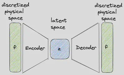
Popular methods to find a low-dimensional embedding on which a given system can be described on include linear methods like the principal component analysis (PCA) (also known as proper orthogonal decomposition (POD)) or its nonlinear counterpart autoencoders (AE). Those methods can be used to find a low-dimensional representation of the discretized vector field

but also to reconstruct the given discretization from this latent vector

In case of an autoencoder, these mappings are found by optimizing the reconstruction loss

for the networks’ weights $\mathbf{\theta}_\text{e}, \mathbf{\theta}_\text{d}$ given some training data. Whereas a truncated singular value decomposition of the training data can be used in case of PCA.

Just as there are different approaches for the reduction, there are also different methods to approximate the temporal dynamics of a system. In case the underlying PDE is known, quasi-Newton solvers for implicit time integration of the latent dynamics on a continuously-differentiable nonlinear manifold have been used in [LeeCarlberg20]. When there is no knowledge about the underling equations present, some of the purely data-driven approaches try to directly approximate the time-dependent latent variable $\mathbf{z}(t) \approx \mathbf{\psi}(t)$ [KneiflEtAl23] (Caution self-promotion), while others try to approximate the right-hand side of an ODE $\mathbf{\dot{z}}(t) = \mathbf{q}(\mathbf{z}, t) \approx \mathbf{\psi}(\mathbf{z}, t)$ on the low-dimensional embedding [ChampionEtAl19]. In both cases, $\mathbf{\psi}(t)$ could be parameterized by a neural network.

What all those approaches share is that they rely on an already discretized vector field. Consequently, a change of resolution requires a new architecture and new training of the reduced order model. Furthermore, they don’t allow adaptive spatial resolution what can be useful in scenarios of varying intensity (low resolution when nothing is happening, high resolution when things get exciting) or for applications under changes of available computational resources. CROM claims to be able to overcome these disadvantages. So, let’s have a look how CROM differs from the previously presented approaches.

CROM

Embedding

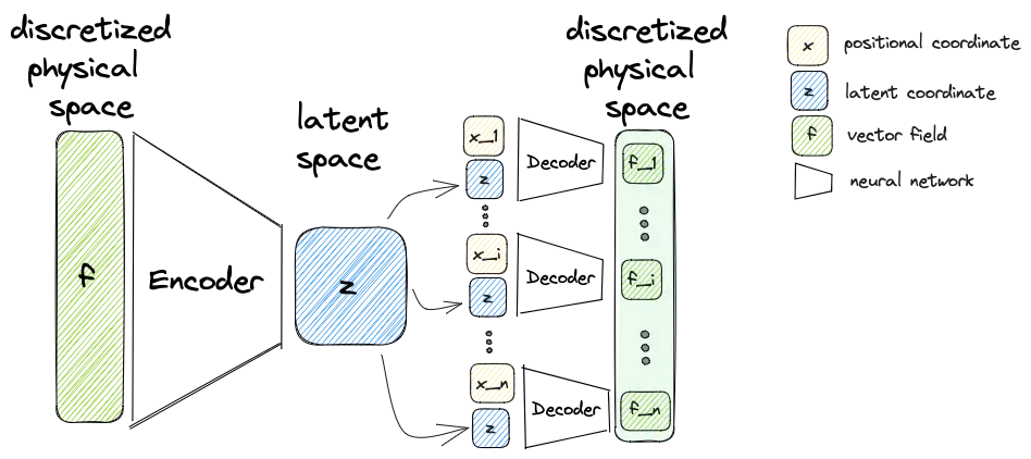
Similar to a conventional autoencoder approaches it constructs an encoder and a decoder. While there are no changes to the encoder compared to conventional methods, the decoder this time does not try to reconstruct a discretized vector field from the latent variable. Instead the decoder

takes the latent variable $\mathbf{z}(t)$ along with the positional variable $\mathbf{x}$ as input to reconstruct the vector field at this certain point. Consequently, the decoder directly approximates the continuous vector field. That’s what the title of the original paper is referring to when speaking of implicit neural representations: Neural representations are class of methods using neural networks to represent arbitrary vector fields.

To reproduce the behavior of a classical autoencoder, the decoder must be evaluated at all points of the discretization with different positional input. However, it is also possible to reconstruct the vector field for any other point $\mathbf{x}\in\Omega$. In order to optimize the weights of the encoder and decoder the loss function (ref) changes to

Dynamics

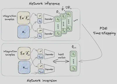
In contrast to conventional approaches CROM, evaluates the actual PDE for a small number of domain points $\mathcal{X}=\{\mathbf{x}^i\}_{i=1}^{m}$ to evolve in time. For a small set, i.e. $m \ll P$, this leads to dramatic time savings compared to the full-order model where the PDE must be evaluated at all $P$ points. The approach to update the latent variable from the current state $\mathbf{z}_{n}=\mathbf{z}(t_{n})$ to the subsequent one $\mathbf{z}_{n+1}=\mathbf{z}(t_{n+1})$ at the next time step consists of three steps:

1. network inference
2. PDE time-stepping
3. network inversion

Network Inference

During the first step of the computation of the latent space dynamics, all spatiotemporal information for the PDE time-stepping is gathered for the selected samples $\mathcal{X}$. The function value itself $\mathbf{f}(\mathbf{x},t_n)=dec(\mathbf{x}, \mathbf{z}_n)$ is obtained from the decoder for all $\mathbf{x}\in\mathcal{X}$along with the spatial $\nabla\mathbf{f}(\mathbf{x},t_n) = \nabla_\mathbf{x}dec(\mathbf{x}, \mathbf{z}_n)$ as well as temporal gradients $\dot{\mathbf{f}}(\mathbf{x},t_n) = \frac{\partial dec(\mathbf{x}, \mathbf{z}_n)}{\partial \mathbf{z}}\dot{\mathbf{z}}_n$. A similar procedure can be used for higher order terms ( $\nabla^2_\mathbf{x}dec(\mathbf{x}, \mathbf{z}_n), \ddot{\mathbf{f}}(\mathbf{x},t_n), \dots $).

PDE Time-stepping

Having all necessary information available, the PDE $\mathcal{F}(\mathbf{f}_n, \nabla\mathbf{f}_n, \dots, \dot{\mathbf{f}}_{n+1}, \dots)=0$ is evolved from $t_n$ to $t_{n+s}$. For each domain point $\mathbf{x}\in\mathcal{X}$, the PDE is solved for the temporal derivative $\dot{\mathbf{f}}_{n+1}$ and the configuration is then evolved in time using a, in this case, explicit time integration method $\mathcal{I}_{\mathcal{F}}$ like Runge-Kutta methods. The update then follows $$\mathbf{f}_{n+1} = \mathcal{I}_{\mathcal{F}}(\Delta t, \mathbf{f}_{n}, \dot{\mathbf{f}}_{n+1}) \quad \forall \mathbf{x}\in\mathcal{X} . $$

Network Inversion

In the last step the dynamics on the reduced manifold are updated in such a way that $\mathbf{z}_{n+1}$ matches best to the just calculated $\mathbf{f}_{n+1}$. To achieve this the optimization problem $$\mathbf{z}_{n+1}^*= \underset{\mathbf{z}_{n+1}}{\text{argmin}} \sum_{\mathbf{x}\in\mathcal{X}} \left| dec(\mathbf{x}, \mathbf{z}_{n+1}) - \mathbf{f}(\mathbf{x}, t_{n+1})\right| $$ is solved with a with Gauss-Newton algorithm or using linearization.

Examples

High-fidelity Model

The high-fidelity spatial vector field is discretized with $P=501$ points and solved using the forward time-centered space method, a finite difference method that is based on the forward Euler method. An update of the vector field thus results in $$ \frac{u_{n+1}^i - u_{n}^i}{\Delta t} = \alpha \frac{u_n^{i+1} - 2u_n^{i} + u_n^{i-1}}{\Delta x^2}\\ \Leftrightarrow \\ u_{n+1}^i = u_n + \frac{\alpha \Delta t}{\Delta x^2}(u_n^{i+1} - 2u_n^{i} + u_n^{i-1}). $$ With this method training and test data is generated based on different diffusion factors $\alpha_1, \alpha_2, \alpha_3 \in [0.0,1.0]^3$. Thereby, the initial condition is the same for every simulation and just the diffusion factors change.

For a given initial condition and values of alpha and it can be solved using the following code snippet

import numpy as np

def solve_diffusion(Nt, Nx, dx, dt, alpha, u_init):
    """
    Solve the diffusion equation u_t - alpha * u_xx = 0 with a first-order Euler scheme
    :param Nt: number of time steps
    :param Nx: number of spatial grid points
    :param dx: spatial step size
    :param dt: time step size
    :param alpha: diffusion coefficient
    :param u_init: initial condition
    :return: u
    """
    # create temperature vector of size (timesteps x spatial points)
    u = np.zeros((Nt, Nx))
    # set initial condition
    u[0] = u_init

    # Main time-stepping loop
    for t in range(1, Nt):
        # Compute the second derivative using finite differences
        u_xx = np.zeros(Nx)
        u_xx[1:Nx-1] = (u[t - 1, 2:] - 2 * u[t - 1, 1:-1] + u[t - 1, :-2]) / (dx ** 2)
        # Update the solution
        u_t = alpha * u_xx
        # update solution using a first-order Euler scheme
        u[t] = u[t - 1] + dt * u_t

    return u

Reduced-Order Model

The latent dimension of the reduced order model is set to $r=16$ and the decoder $dec(x, \mathbf{z})$ consists out of three fully-connected hidden layers with 128 neurons each.

A very simple implementation of the autoencoder for this example in PyTorch could look like this:

import torch
from torch import nn

# create autoencoder
class CROMAutoencoder(nn.Module):
    def __init__(self, r, n_x, n_d=1, n_layers=1, n_neurons=128):
        """
        :param r: latent space dimension
        :param n_x: number of spatial points
        :param n_d: number of coordinates required to describe the position (1 for 1D, 2 for 2D, ...)
        :param n_layers: number of hidden layers in the encoder and decoder
        :param n_neurons: number of neurons in each hidden layer
        """
        super(CROMAutoencoder, self).__init__()
        self.r = r
        self.n_x = n_x
        self.n_d = n_d
        self.n_layers = n_layers
        self.n_neurons = n_neurons

        # create layers for the encoder
        self.encoder_0 = nn.Linear(self.n_x, self.n_neurons)
        self.encoder_0_act = nn.ELU(True)
        # hidden layers
        for i in range(n_layers):
            setattr(self, f'encoder_{i + 1}', nn.Linear(self.n_neurons, self.n_neurons))
            setattr(self, f'encoder_{i + 1}_act', nn.ELU(True))
        setattr(self, f'encoder_{n_layers + 1}', nn.Linear(self.n_neurons, self.r))

        # create layers for decoder
        self.decoder_0 = nn.Linear(self.r + self.n_d, self.n_neurons)
        self.decoder_0_act = nn.ELU(True)
        # hidden layers
        for i in range(n_layers):
            setattr(self, f'decoder_{i + 1}', nn.Linear(self.n_neurons, self.n_neurons))
            setattr(self, f'decoder_{i + 1}_act', nn.ELU(True))
        # output layer with skip connection from spatial coordinate
        setattr(self, f'decoder_{n_layers + 1}', nn.Linear(self.n_neurons + self.n_d, 1))

    def encoder(self, u):
        """
        Encoder that maps the vector field values to the latent space
        :param u: (batchsize x n) vector field values
        :return:
        """
        for i in range(self.n_layers+2): # +2 for input and output layer
            u = getattr(self, f'encoder_{i}')(u)
            if hasattr(self, f'encoder_{i}_act'):
                u = getattr(self, f'encoder_{i}_act')(u)
        return u

    def decoder(self, x, z):
        """
        Decoder that maps the latent variable along with a spatial coordinate to the reconstructed vector field value
        :param x: (batchsize x n) positional coordinates
        :param z: (batchsize x r) latent variable
        :return:
        """

        # save batch size for reshaping later
        batch_size_local = x.size(0)

        # repeat z for every point in x (batch_size_local x n_x x r)
        z = z.unsqueeze(1).repeat(1, x.size(1), 1)
        # add new axis to x to the end (batch_size_local x n_x x n_d)
        x = x.unsqueeze(2)
        # concatenate x and z
        decoder_input = torch.cat((x, z), dim=2)
        # reshape for decoder so that all the points are processed at once (batchsize = batch_size_local * n_x)
        decoder_input = decoder_input.view(-1, self.r + self.n_d)

        u_ = decoder_input
        for i in range(self.n_layers + 1): # +1 for input layer
            u_ = getattr(self, f'decoder_{i}')(u_)
            if hasattr(self, f'decoder_{i}_act'):
                u_ = getattr(self, f'decoder_{i}_act')(u_)
        # stack x and u_ (skip connection from x to output layer)
        output_input = torch.cat((x.view(-1, self.n_d), u_), dim=1)
        u_ = getattr(self, f'decoder_{self.n_layers + 1}')(output_input)

        # reshape x_rec
        u_rec = u_.view(batch_size_local, -1)

        return u_rec

    def forward(self, x, u):
        """
        :param x: (batchsize x n) positional coordinates
        :param u: (batchsize x n) vector field values
        """

        # encode input to latent space
        z = self.encoder(u)

        # reshape x_rec
        u_rec = self.decoder(x, z)

        return u_rec

In contrast to the implementation of the original paper, I don’t use convolutional layers for simplicity and introduced a skip-connection in the decoder from the spatial coordinate $x$ to the output layer to facilitate the network’s ability to recognize spatial dependencies. This autoencoder can then be trained on the FOM simulation data to find the low-dimensional embedding. After 12000 epochs, the autoencoder is able to reconstruct the full vector field quite well as demonstrated in the following gif.

Hereafter, we can evolve the latent dynamics in time using only a few (in this case $m=22$) integration points. For a guidance how to select those points, please refer to the original paper.

def time_stepping(model, n_t, n_x, dt, x_support, support_point_indices, alpha_support, u_init):
    """
    Time evolution of the latent variable by evaluating the original PDE on a small number of support points
    and then finding the latent variables that matches best to the found evolved vector field values
    :param model: CROMAutoencoder model
    :param n_t: number of time steps
    :param n_x: number of spatial grid points
    :param dt: time step size
    :param x_support: spatial grid points that are evaluated during time stepping
    :param support_point_indices: indices of the support points
    :param alpha_support: diffusion coefficients at the support points
    :param u_init: initial condition of the vector field
    :return:
    """
    # encode initial condition
    z_init = model.encoder(torch.from_numpy(u_init).float()).detach().requires_grad_()
    # create latent vector of size (timesteps x (spatial points + 1))
    z = torch.zeros((n_t, model.r))
    # set initial condition
    z[0] = z_init
    # Main time-stepping loop
    for i_time in range(1, n_t):
        # compute the second order spatial gradient using autograd
        hessian = torch.func.hessian(model.decoder, argnums=0)(x_support, z[i_time-1:i_time]).squeeze()
        u_xx = torch.diagonal(torch.diagonal(hessian, dim1=0, dim2=1), dim1=0, dim2=1).detach().squeeze()
        # apply boundary conditions
        for i, index in enumerate(support_point_indices):
            if index == 0 or index == n_x:
                u_xx[i] = 0

        # get time derivative
        u_t = alpha_support * u_xx

        # evolve latent variable in time (this part uses the linearized version instead of Gauss-Newton solver)
        res = u_t
        jac = torch.func.jacrev(model.decoder, argnums=1)(x_support, z[i_time-1:i_time]).detach().squeeze()
        vhat = torch.inverse(torch.matmul(jac.transpose(1, 0), jac)).matmul(jac.transpose(1, 0)).matmul(res)
        vhat = vhat.view(1, 1, -1)  # (dim: ? x ? x r)
        z[i_time] = z[i_time-1] + vhat * dt

    return z

From this latent time series, we can reconstruct the full vector field at arbitrary points $x\in\Omega$. An example result for a test scenario can be seen in the following gif.

Concluding Remarks

CROM is a very powerful discretization-free ROM scheme for PDEs. The authors showed that it can outperform conventional approaches regarding accuracy and resource demands while offering adaptive spatial resolutions. Nevertheless, it shares some limitations with classic data-driven ROM approaches like the dependency on the training data, i.e. it won’t generalize well to unseen scenarios. In contrast to complete data-driven approaches it offers a nice blend of ML and PDE solutions at the cost of increased method complexity.

Should you use CROM?

Well, it depends. It is a very promising method which is likely to pave the way for many more great research projects. Especially, when you can take advantage of adaptively adjusting your discretization ,it is worth a try. If you, however, don’t mind the discretization present in your problem, you can still go for the more conventional approaches and in that case even consider whether linear reduction (PCA) isn’t suitable for your certain problem.

Did you find this page helpful? Consider sharing it 🙌