VENI, VINDy, VICI

Complex physical systems — think fluid flows, structural vibrations, or chemical reactions — are typically modeled by partial differential equations (PDEs). Solving these PDEs numerically is accurate but expensive: a single simulation can take hours or days. Reduced-order models (ROMs) or deep learning surrogate models tackle this by finding a low-dimensional representation of the system that is cheap to evaluate. The catch is that most ROMs are deterministic and assume clean, reliable data, neither of which holds in practice; while data-driven approaches often lack interpretability.

VENI, VINDy, VICI [paper] addresses those issues at once. It builds a generative ROM that (1) handles noisy input data, (2) identifies interpretable governing equations in a low-dimensional space, and (3) produces predictions with calibrated uncertainty estimates — all within a single probabilistic framework.

---

The Big Picture

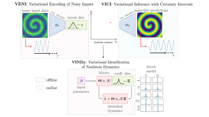
The framework consists of three tightly coupled components:

• VENI — Variational Encoding of Noisy Inputs: compress high-dimensional, noisy state snapshots into a low-dimensional probabilistic latent space using a variational autoencoder.
• VINDy — Variational Identification of Nonlinear Dynamics: discover sparse governing equations in the latent space, where the equation coefficients are themselves probability distributions.
• VICI — Variational Inference with Certainty Intervals: propagate both latent dynamics and the coefficient uncertainty forward in time to produce predictions with confidence bounds.

What sets this apart from standard ROMs is that uncertainty is embedded into every step, from the encoding of raw data all the way to the final prediction.

---

VENI: Encoding with a Variational Autoencoder

A standard autoencoder maps each input snapshot $\mathbf{x} \in \mathbb{R}^N$ to a single point $\mathbf{z} \in \mathbb{R}^n$ in a low-dimensional latent space ( $n \ll N$). This works well for clean data, but when measurements are noisy, the encoder has no principled way to separate signal from noise.

A variational autoencoder (VAE) takes a different approach: instead of mapping to a point, the encoder $\boldsymbol{\phi}$ maps each input to a distribution over the latent space,

$$ q_{\boldsymbol{\phi}}(\mathbf{z} \mid \mathbf{x}) = \mathcal{N}\!\left( \boldsymbol{\mu}_{\boldsymbol{\phi}}(\mathbf{x}),\, \text{diag}(\boldsymbol{\sigma}^2_{\boldsymbol{\phi}}(\mathbf{x}))\right). $$

Concretely, the encoder network outputs two vectors — a mean $\boldsymbol{\mu}$ and a standard deviation $\boldsymbol{\sigma}$ — for every input snapshot. A latent state is then sampled from this Gaussian rather than being read off directly. The decoder takes this sample and reconstructs the full-dimensional state.

Training maximises the evidence lower bound (ELBO), where a reconstruction term encourages the decoder to faithfully recover the input and the KL divergence pulls the learned posteriors towards a standard Gaussian prior (see paper for details). The balance between the two forces the latent space to be both informative and smooth — any noise in the input is naturally absorbed by the width of the posterior.

The practical effect is elegant: clean snapshots get narrow posteriors (the encoder is confident about where they live in the latent space), while noisy or ambiguous snapshots get wider posteriors (the encoder admits its uncertainty). This propagates naturally into downstream uncertainty estimates.

---

VINDy: Identifying Dynamics as Distributions

From SINDy to VINDy

Once we have a low-dimensional latent trajectory $\mathbf{z}(t) \in \mathbb{R}^n$, we want to find the governing equations of its dynamics. SINDy (Sparse Identification of Nonlinear Dynamics) does this by assuming the right-hand side of the latent ODE is a sparse linear combination of candidate functions:

$$ \dot{\mathbf{z}}(t) = \boldsymbol{\Xi}\,\boldsymbol{\Theta}(\mathbf{z}), $$

where $\boldsymbol{\Theta}(\mathbf{z}) = [1,\, z_1,\, z_2,\, z_1^2,\, z_1 z_2,\, \dots] \in \mathbb{R}^{r} $ is a library of candidate functions and $\boldsymbol{\Xi} \in \mathbb{R}^{n \times r}$ is a sparse coefficient vector — most entries are zero, meaning only a handful of terms actually drive the dynamics. This sparsity makes the identified model interpretable: we get an explicit equation rather than a black-box neural network.

Standard SINDy fits a single coefficient vector, which is fine for clean data but fragile in the presence of noise: small errors in $\dot{\mathbf{z}}$ can corrupt the identified equations.

VINDy replaces the point-estimate coefficients with distributions:

$$ \boldsymbol{\Xi}_i \sim \mathcal{L}(\mu_i, \sigma_i^2), \quad i = 1, \dots, n_\text{lib}. $$

Each coefficient is now a Gaussian $\mathcal{N}$ or Laplacian $\mathcal{L}$ distribution parametrized by a learnable location $\mu_i$ and scaling factor $\sigma_i$. A coefficient with a large mean and small variance corresponds to a term that is confidently important. A coefficient near zero with large variance corresponds to a term that could be pruned — the model is uncertain whether it belongs in the equation at all.

Training

VINDy is trained jointly with the VAE by adding a dynamics term to the ELBO. Latent states $\mathbf{z}(t)$ are sampled from the VAE encoder, latent time derivatives $\dot{\mathbf{z}}$ are computed via the chain rule, and the coefficient distributions are optimized so that $\boldsymbol{\Xi}\,\boldsymbol{\Theta}(\mathbf{z})$ matches $\dot{\mathbf{z}}$ in expectation. A sparsity-promoting prior (analogous to the KL term in the VAE) further encourages most coefficients to shrink to zero, recovering interpretable, parsimonious dynamics.

The animation above captures the key behaviour: as training progresses, most coefficient distributions collapse towards zero while a small subset converge to confident, non-zero values — the framework automatically discovers which terms matter.

---

VICI: Predictions with Uncertainty Intervals

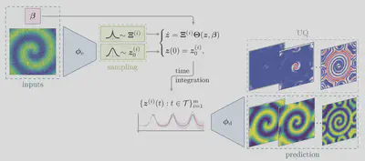
With a trained VAE and a distribution over governing equations in hand, making predictions is straightforward:

1. Sample multiple coefficient vectors $\boldsymbol{\Xi}^{(k)} \sim \mathcal{L}(\boldsymbol{\mu}_\Xi, \text{diag}(\boldsymbol{\sigma}^2_\Xi))$ and latent initial conditions $\boldsymbol{z}^{(k)}_0 \sim \mathcal{N}\!\left( \boldsymbol{\mu}_{\boldsymbol{\phi}}(\mathbf{x}),\, \text{diag}(\boldsymbol{\sigma}^2_{\boldsymbol{\phi}}(\mathbf{x}))\right)$.
2. Integrate the latent ODEs $\dot{\mathbf{z}} = \boldsymbol{\Xi}^{(k)}\,\boldsymbol{\Theta}(\mathbf{z})$ forward from the latent initial conditions, giving a bundle of latent trajectories $\{\mathbf{z}^{(k)}(t)\}$.
3. Decode each trajectory back to the full state space using the VAE decoder.
4. Summarise the resulting ensemble: the mean is the point prediction; the spread gives the uncertainty interval.

This yields not just a single trajectory but a predictive distribution over future states. The uncertainty grows naturally for longer horizons or when the initial condition lies away from the training distribution — precisely the situations where a user most needs to know how much to trust the model.

Two sources of uncertainty are represented separately and propagate independently:

• Data noise (captured by $\boldsymbol{\sigma}^2_{\boldsymbol{\phi}}$ of the VAE encoder)
• Model uncertainty (captured by $\boldsymbol{\sigma}^2_\Xi$ of the VINDy coefficients)

---

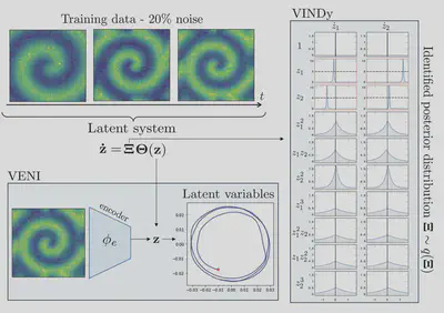
Example: Reaction–Diffusion System

We applied VENI, VINDy, VICI among others to a reaction–diffusion system that generates rotating spiral waves — a PDE with rich spatio-temporal dynamics that lives on a genuinely low-dimensional manifold.

The full state is a spatial grid with thousands of degrees of freedom. The framework compresses this to just two latent variables, finds an interpretable oscillatory equation governing their interaction via VINDy, and uses VICI to predict future states together with uncertainty bounds — closely matching the high-fidelity simulation while providing a measure of confidence in the prediction.

The latent dynamics take the form of a simple nonlinear oscillator, and the VINDy coefficients cleanly identify the relevant coupling terms. This interpretability is a direct consequence of the sparse probabilistic identification: rather than a black-box neural ODE, we obtain an equation we can inspect, simulate cheaply, and reason about physically.

---

Why Does This Matter?

Property	Standard ROM	VENI, VINDy, VICI
Handles noisy data	✗	✓
Interpretable dynamics	Partial	✓ (sparse equations)
Uncertainty quantification	✗	✓ (end-to-end)
Generative	✗	✓
Works without knowledge of PDE	(✓)	✓

The combination of interpretability and probabilistic uncertainty quantification is what distinguishes this approach. An engineer using the model gets not just a fast surrogate, but also an explicit equation and a principled confidence estimate — both critical for any safety-relevant application.

---

Did you find this page helpful? Consider sharing it!